After learned variational inference and latent dirichlet allocation (LDA), I wrote a paper about Gaussian relational topic model to solve the problem of connection discovery using shared images. In order to continue solving more challenging problems and improving myself, I find it necessary to master Markov Chain Monte Carlo methods. Therefore, I put my hands on Gibbs sampling and Metropolis Hastings algorithm.

Gibbs Sampling and Collapsed Gibbs Sampling

The basic idea is to sample each variable in turn, conditioned on the values of all the other variables:

The ideal of collapsed Gibbs sampling is to integrate out all possible model parameters analytically, such that the sampling space is minimum, dramatically decrease sampling time. An example of collapsed Gibbs sampling for fitting a GMM can be found in Murphy’s book, p. 844. The example code of collapsed Gibbs sampling solving Bayesian Gaussian mixture model can be found in here. The main logic of the collapsed Gibbs sampling is:

# Loop over iterations
for i_iter in range(n_iter):

    # Loop over data items
    for i in xrange(self.components.N):

        # Cache some old values for possible future use
        k_old = self.components.assignments[i]
        K_old = self.components.K
        stats_old = self.components.cache_component_stats(k_old)

        # Remove data vector `X[i]` from its current component
        self.components.del_item(i)

        # Compute log probability of `X[i]` belonging to each component
        # (24.26) in Murphy, p. 843
        log_prob_z = (
            np.ones(self.components.K_max)*np.log(
                float(self.alpha)/self.components.K_max + self.components.counts
                )
            )
        # (24.23) in Murphy, p. 842
        log_prob_z[:self.components.K] += self.components.log_post_pred(i)
        # Empty (unactive) components
        log_prob_z[self.components.K:] += self.components.log_prior(i)
        prob_z = np.exp(log_prob_z - logsumexp(log_prob_z))

        # Sample the new component assignment for `X[i]`
        k = utils.draw(prob_z)

        # There could be several empty, unactive components at the end
        if k > self.components.K:
            k = self.components.K
        # print prob_z, k, prob_z[k]

        # Add data item X[i] into its component `k`
        if k == k_old and self.components.K == K_old:
            # Assignment same and no components have been removed
            self.components.restore_component_from_stats(k_old, *stats_old)
            self.components.assignments[i] = k_old
        else:
            # Add data item X[i] into its new component `k`
            self.components.add_item(i, k)

    # Update record
    record_dict["sample_time"].append(time.time() - start_time)
    start_time = time.time()
    record_dict["log_marg"].append(self.log_marg())
    record_dict["components"].append(self.components.K - 1)

    # Log info
    info = "iteration: " + str(i_iter)
    for key in sorted(record_dict):
        info += ", " + key + ": " + str(record_dict[key][-1])
    info += "."
    logger.info(info)

Metroplis Hastings and Slice Sampling

As an experiment of Metroplis Hastings algorithm, I find this link useful. It also compares Metropolis Hastings with slice sampling, both are worth investigating. Following experiments are based on the post.

Anyway, first let’s describe the model we are going to MCMC with. It’s a two level hierachical model:

The joint distribution is obviously given by

The class defining the distribution for sampling and probability density evaluation is given:

from __future__ import division

import numpy as np
import scipy.stats as ss


class joint_dist(object):

    def rvs(self, n=1):
        """ sample a random variable from this distribution """
        sample = np.zeros((10, n))

        for i in xrange(n):
            # generate rvs
            v = ss.norm(0, 3).rvs()
            xs = ss.norm(0, np.sqrt(np.e**v)).rvs(9)
            # place in sample array
            sample[0, i] = v
            sample[1:, i] = xs

        return sample

    def pdf(self, sample):
        """ get the probability of a specific sample """
        v = sample[0]
        pv = ss.norm(0, 3).pdf(v)
        xs = sample[1:]
        pxs = [ss.norm(0, np.sqrt(np.e**v)).pdf(x_k) for x_k in xs]
        return np.array([pv] + pxs)

    def loglike(self, sample):
        """ log likelihood of a specific sample """
        return np.sum(np.log(self.pdf(sample)))

The current state is defined as $w=[v,x_1,x_2,…,x_9]$. And the proposal funciton is defined as symmetric normal distribution with the current state as mean:

The Metropolis-Hasting function is defined:

def metropolis(init, iters):
    """
    based on http://www.cs.toronto.edu/~asamir/cifar/rpa-tutorial.pdf
    
    can take several minutes to run with large sample sizes.
    """
    dist = joint_dist()

    # set up empty sample holder
    D = len(init)
    samples = np.zeros((D, iters))

    # initialize state and log-likelihood
    state = init.copy()
    Lp_state = dist.loglike(state)

    accepts = 0
    for i in np.arange(0, iters):
        
        # propose a new state
        prop = np.random.multivariate_normal(state.ravel(), np.eye(10)).reshape(D, 1)

        Lp_prop = dist.loglike(prop)
        rand = np.random.rand()
        if np.log(rand) < (Lp_prop - Lp_state):
            accepts += 1
            state = prop.copy()
            Lp_state = Lp_prop

        samples[:, i] = state.copy().ravel()
        
        if i % 1000 == 0: print('[#iter: %d]' %i)

    print 'Acceptance ratio', accepts/iters
    return samples

Let’s start by taking 50,000 samples using Metropolis-Hastings.

# define our starting point
w_0 = np.array([0., 1., 1., 1., 1., 1., 1., 1., 1., 1.])

# actually do the sampling
n = 50000
samples = metropolis(w_0, n)

Acceptance ratio 0.24342

import matplotlib.pyplot as plt
%matplotlib inline  
from matplotlib import rcParams
rcParams['font.size'] = 12
rcParams['figure.figsize'] = (10, 6)

burnin = 10000
m = n-burnin
v = samples[0, burnin:]
fig = plt.figure()
ax0 = fig.add_subplot(211)
#fig, (ax0, ax1) = plt.subplots(2, 1)

# show values of sampled v by iteration
ax0.plot(np.arange(m), v)
ax0.set_xlabel('iteration number')
ax0.set_ylabel('value of sampled v')

ax1 = fig.add_subplot(212)
# plot a histogram of values of v
ax1.hist(v, bins=80)
ax1.set_xlabel('values of sampled v')
ax1.set_ylabel('observations')

plt.show()

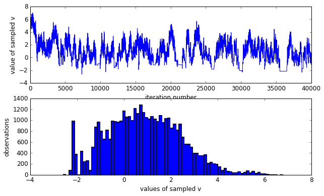
As it should be noticed that the sampled $v$ is not Gaussian distributed, rather skewed. However, we know that $v$ is in fact zero-mean gaussian distributed. The skewed sampling is not good to estimate the true distribution of $v$. As discussed in the original post, it is because under the directed regime — any small or negative $v$ implies that every $x_k∼\mathcal{N}(0,e^v \approx 0)$, thus imposing a huge probability “penalty” on any non-zero $x_k$. Meanwhile, our Metropolis-Hastings is naively proposing a vector of $x_k$s which are probably not all zero, so we tend to reject any small or negative $v$.

So for slice sampling:

def slice_sample(init, iters, sigma, step_out=True):
    """
    based on http://homepages.inf.ed.ac.uk/imurray2/teaching/09mlss/
    sigma is the step size of each coordinate
    """

    dist = joint_dist()

    # set up empty sample holder
    D = len(init)
    samples = np.zeros((D, iters))

    # initialize
    xx = init.copy()

    for i in xrange(iters):
        perm = range(D)
        np.random.shuffle(perm)
        last_llh = dist.loglike(xx)

        # Sweep through axes (simplest thing)
        for d in perm:
            # u|x ~ [0,1]*p(x)
            llh0 = last_llh + np.log(np.random.rand())
            
            # Create a horizontal interval (x_l, x_r) enclosing xx
            rr = np.random.rand(1)
            x_l = xx.copy()
            x_l[d] = x_l[d] - rr * sigma[d]
            x_r = xx.copy()
            x_r[d] = x_r[d] + (1 - rr) * sigma[d]

            # step out p(x)>u'
            if step_out:
                llh_l = dist.loglike(x_l)
                while llh_l > llh0:
                    x_l[d] = x_l[d] - sigma[d]
                    llh_l = dist.loglike(x_l)
                llh_r = dist.loglike(x_r)
                while llh_r > llh0:
                    x_r[d] = x_r[d] + sigma[d]
                    llh_r = dist.loglike(x_r)

            x_cur = xx.copy()
            while True:
                xd = np.random.rand() * (x_r[d] - x_l[d]) + x_l[d]
                x_cur[d] = xd.copy()
                last_llh = dist.loglike(x_cur)
                if last_llh > llh0: #this is the only way to leave the while loop, satiesfy p(x)>u'
                    xx[d] = xd.copy()
                    break
                elif xd > xx[d]:
                    x_r[d] = xd
                elif xd < xx[d]:
                    x_l[d] = xd
                else:
                    raise RuntimeError('Slice sampler shrank too far.')

        if i % 1000 == 0: print 'iteration', i

        samples[:, i] = xx.copy().ravel()

    return samples

# define our starting point
w_0 = np.array([0., 1., 1., 1., 1., 1., 1., 1., 1., 1.])

# actually do the sampling
n = 10000
sigma = np.ones(10)
samples = slice_sample(w_0, iters=n, sigma=sigma)

burnin = 0
m = n-burnin
v = samples[0, burnin:]
fig = plt.figure()
ax0 = fig.add_subplot(211)
#fig, (ax0, ax1) = plt.subplots(2, 1)

# show values of sampled v by iteration
ax0.plot(np.arange(m), v)
ax0.set_xlabel('iteration number')
ax0.set_ylabel('value of sampled v')

ax1 = fig.add_subplot(212)
# plot a histogram of values of v
ax1.hist(v, bins=80)
ax1.set_xlabel('values of sampled v')
ax1.set_ylabel('observations')

plt.show()