Stochastic Gradient Monte Carlo
Lately, I’m trying to investigate Bayesian Deep Learning and seriously considering it to be my PhD topic. Combining Bayesian with Deep Learning is current hot topic and with the current development of stochastic gradient monte carlo, I think it’s time for Bayesian Deep Learning to fly. And I could probably benefit from it a lot.
Hamiltonian Monte Carlo
A perfect tutorial for introduction of Hamiltonian Monte Carlo is MCMC: Hamiltonian Monte Carlo (a.k.a. Hybrid Monte Carlo).
Stochastic Gradient Monte Carlo
Here, I’m going to run some examples using Hamiltonian Monte Carlo, Stochastic Gradient Langevin Dynamics and Stochastic Gradient Hamiltonian Monte Carlo.
Suppose we are dealing with target distribution of
Think of it as the un-normalized log probability of
Then the un-normalized posterior of $\theta$ is given by:
And the true gradient is
However, if stochastic gradient noise, the gradient we get by calculating stochastic gradient would have an additional noise term. Let’s define the noisy gradient as
Let’s see how we can approximate this target distribution with noisy gradient using monte carlo methods.
%matplotlib inline

import numpy as np
import matplotlib.pyplot as plt

nsample = 80000;
xStep = 0.1;
m = 1;
C = 3;
dt = 0.1;
nstep = 50;
V = 4;

#set random seed
np.random.seed(10);

def U(x):
    return -2 * x**2+x**4
def gradU(x):
    return -4*x+4*x**3+np.random.randn()*2
def gradUPerfect(x):
    return -4*x+4*x**3
#draw probability diagram
xGrid = np.array(np.arange(-2,2,xStep));
y = np.exp( - U(xGrid) ); # take exponential to convert from log to un-normalized probability
y = y / sum(y) / xStep; # normalize, then divided by xStep to calculate the density
# "Gold Standard" Hamiltonian Monte Carlo
def hmc( U, gradU, m, dt, nstep, x, mhtest ):
    # HMC using gradU, for nstep, starting at position x
    p = np.random.randn() * np.sqrt( m );
    oldX = x;
    oldEnergy = p * m * p / 2 + U(x);
    # do leapfrog
    for i in range(nstep):
        p = p - gradU( x ) * dt / 2;
        x = x + p/m * dt;
        p = p - gradU( x ) * dt / 2;

    p = -p;

    # M-H test
    if mhtest != 0:
        newEnergy  = p * m * p / 2 + U(x);
        if np.exp(oldEnergy- newEnergy) < np.random.rand():
            # reject
            x = oldX;
    return x

# HMC without noise with M-H
samples = np.zeros(nsample);
x = 0;
for i in range(nsample):
    x = hmc( U, gradUPerfect, m, dt, nstep, x, 1); # no stochastic gradient noise
    samples[i] = x;

[yhmc,xhmc] = np.histogram(samples, xGrid);
yhmc = 1.0 * yhmc / np.sum(yhmc) / xStep;
# Stochastic Gradient Langevin Dynamics
def sgld( U, gradU, m, dt, nstep, x, C, V ):
    # vanilla SGLD using gradU, for L steps, starting at position x
    sigma = np.sqrt( 2 * dt);
    for t in range(nstep):
        dx = - gradU( x ) * dt + np.random.randn() * sigma;
        x = x + dx;
# SGHMC with noise, no M-H
samples = np.zeros(nsample);
x = 0;
for i in range(nsample):
    x = sghmc( U, gradU, m, dt, nstep, x, C, V );
    samples[i] = x;

ysgld,xsgld = np.histogram(samples, xGrid);
ysgld = 1.0 * ysgld / sum(ysgld) / xStep;
# Stochastic Gradient Hamiltonian Monte Carlo
def sghmc( U, gradU, m, dt, nstep, x, C, V ):
    # SGHMC using gradU, for nstep, starting at position x
    p = np.random.randn() * np.sqrt( m );
    B = 0.5 * V * dt;
    D = np.sqrt( 2 * (C-B) * dt );

    for i in range(nstep):
        p = p - gradU( x ) * dt  - p * C * dt  + np.random.randn()*D;
        x = x + p/m * dt;
    return x

# SGHMC with noise, no M-H
samples = np.zeros(nsample);
x = 0;
for i in range(nsample):
    x = sghmc( U, gradU, m, dt, nstep, x, C, V );
    samples[i] = x;

ysghmc,xsghmc = np.histogram(samples, xGrid);
ysghmc = 1.0 * ysghmc / sum(ysghmc) / xStep;
# plot the approximated distribution
plt.plot(xGrid,y,'-',xhmc[1:],yhmc,'g-v',xsgld[1:], ysgld, 'm-x', xsghmc[1:],ysghmc,'r')
plt.legend( ('True Distribution', 'Standard HMC', 'SGLD', 'SGHMC'), loc='center left', bbox_to_anchor=(1, 0.5))
<matplotlib.legend.Legend at 0x1064ea110>
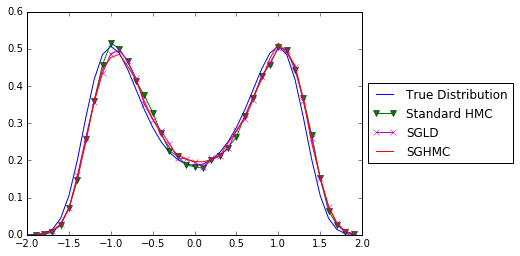
That’s great. We now know that under stochastic gradient noise, we can still approximate the true posterior distribution using monte carlo methods, i.e. SGLD and SGHMC.
Logistic Regression using Stochastic Gradient Monte Carlo
Now let’s do the simplest case, logistic regression. Hope we can see how stochastic gradient monte carlo actually can be applied to real machine learning problem.
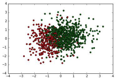
First, let’s construct a toy dataset. We draw our $X$ data from a 2-D normal distribution, $\mathcal{N}(\mu,\Sigma)$.
import numpy as np
import matplotlib.pyplot as plt
import matplotlib

# Setting for data simulation
N = 1000; # data size
D = 3; # parameter size
#betaTrue = np.random.randint(-1, 2, size=(D,1));
betaTrue = np.array([2,3,1]).T

# Add correlation to design matrix X
muDesg = np.zeros(D-1);
corrX = 0.2;
SigmaDesg = np.zeros((D-1,D-1));
for i in range(D-1):
    for j in range(i,D-1):
        SigmaDesg[i,j] = corrX ** (j-i);
        SigmaDesg[j,i] = SigmaDesg[i,j];

X = np.hstack((np.ones((N,1)),np.random.multivariate_normal(muDesg,SigmaDesg,N)));
probTrue = np.exp(np.dot(X, betaTrue))/(1+np.exp(np.dot(X, betaTrue)));
y = np.zeros(N);
for j in range(N):
    y[j] = np.random.binomial(1,probTrue[j]);

NTest = 1000
XTest = np.hstack((np.ones((NTest,1)),np.random.multivariate_normal(muDesg,SigmaDesg,NTest)));
probTrueTest = np.exp(np.dot(XTest, betaTrue))/(1+np.exp(np.dot(XTest, betaTrue)));
yTest = np.zeros(NTest);
for j in range(NTest):
    yTest[j] = np.random.binomial(1,probTrueTest[j]);

cmap, norm = matplotlib.colors.from_levels_and_colors([0, 1, 2], ['red', 'green'])
plt.scatter(X[:,1], X[:,2], c=y, cmap=cmap)
<matplotlib.collections.PathCollection at 0x10cb79b50>
Next, let’s see how each of the methods above can perform logistic regression on this dataset. Here we use prior of normal distribution for $\beta$:
For logistic regression, we have following distribution:
Let’s use SGD as baseline.
Logistic Regression with SGD
# SGD
def prob(w,X):
    return 1.0/(1+np.exp(-X.dot(w)))

def cost(w,X,y,r):
    return -np.sum(y*np.log(prob(w,X))+(1-y)*np.log(1-prob(w,X))) + r * np.dot(w.T,w) /2

def grad(w,X,y,r):
    return -np.dot(X.T,y-prob(w,X)) + r * w

w = np.random.rand(3)
r = 0.1
i = 0
lr = 1e-3
while np.linalg.norm(grad(w,X,y,r)) > 1e-6:
    if i % 1000 == 0:
        print('[Iter %d]: cost=%f' % (i,cost(w,X,y,r)))
    w = w - lr*grad(w,X,y,r)
    i += 1
print "weight: ", w[0],w[1],w[2]
[Iter 0]: cost=605.040794
[Iter 1000]: cost=278.583159
weight:  2.02798388293 3.42836274096 0.931072930232
# Prediction results for SGD
accSGLD = np.mean((prob(w, XTest) > 0.5) == yTest);
print('The test accuracy is %f' % accSGLD)
The test accuracy is 0.855000
Logistic Regression with SGLD
# Stochastic Gradient Langevin Dynamics
import scipy.special
def logistic_function(x):
return .5 * (1 + np.tanh(.5 * x))
def LR_SGLD(X,y):
maxIter = 10000;
# plot index
plotInd = 1;
N, D = X.shape; # data size
tau = int(np.floor(np.sqrt(N))); # size of minibatch
# step size
# a = 1;
# b = 1;
# gamma = 0.7;
# prior
muStar = np.zeros(D);
sigma = 0.1;
SigmaStar = np.eye(D)*sigma;
invSigmaStar = np.linalg.inv(SigmaStar);
# Initialize
beta0 = np.random.rand(D);
betaVec = np.zeros((maxIter,D));
betaVec[0,:] = beta0;
eta = np.zeros(maxIter);
z = np.zeros((maxIter,D));
eta0 = 0.01;
# sgld iteration
for t in range(maxIter-1):
# random sample a minibatch
S = np.random.choice(N,tau, replace=False);
# sample coordinates of z
# eta(t) = a*(b+t)^(-gamma);
eta[t] = max(1/(t+1),eta0);
zVar = eta[t] * 2;
z[t,:] = np.random.randn(D) * np.sqrt(zVar);
gradR = np.dot(invSigmaStar,(betaVec[t,:]-muStar));
#print gradR
gradL = -np.dot(X[S,:].T,(y[S]-scipy.special.expit(np.dot(X[S,:],betaVec[t,:]))));
#print gradL
betaVec[t+1,:] = betaVec[t,:]-eta[t]*(gradR+N/tau*gradL)+z[t,:];
#print betaVec[t+1,:]
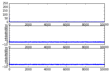
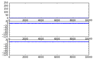
if plotInd == 1:
fig = plt.figure();
ax1 = fig.add_subplot(311)
ax1.plot(range(maxIter),betaVec[:,1]);
ax2 = fig.add_subplot(312)
ax2.plot(range(maxIter),betaVec[:,2]);
ax3 = fig.add_subplot(313)
ax3.plot(range(maxIter),betaVec[:,2]);
burnIn = int(0.5*maxIter);
samples = betaVec[burnIn+1:,:];
return samples
samples = LR_SGLD(X,y)
np.mean(samples,0)
array([ 1.51066479, 2.60689302, 0.77643745])
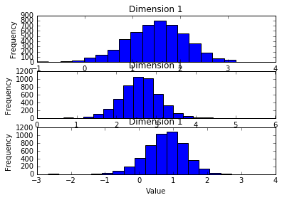
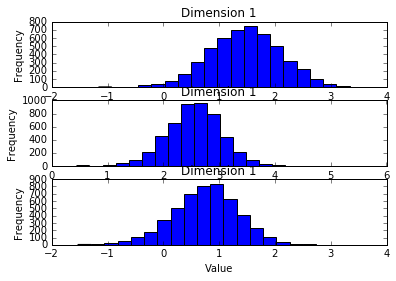
plt.subplot(311)
plt.hist(samples[:,0],20)
plt.title("Dimension 1")
plt.xlabel("Value")
plt.ylabel("Frequency")
plt.subplot(312)
plt.hist(samples[:,1],20)
plt.title("Dimension 1")
plt.xlabel("Value")
plt.ylabel("Frequency")
plt.subplot(313)
plt.hist(samples[:,2],20)
plt.title("Dimension 1")
plt.xlabel("Value")
plt.ylabel("Frequency")
<matplotlib.text.Text at 0x10bc85f10>
# Prediction results for SGLD
betaSamples = samples;
probPred = np.mean(scipy.special.expit(np.dot(XTest,betaSamples.T)),1);
#loglikSGLD(l) = sum(yTest.*log(probPred)+(1-yTest).*log(1-probPred));
accSGLD = np.mean((probPred > 0.5) == yTest);
print('Test accuracy is %f' %accSGLD)
Test accuracy is 0.853000
As it can be seen, using SGLD with minibatch of only about 30, we can approximate the true posterior. Furthermore, as interested by many recent papers, from the posterior distribution of the parameters, we can obtain the uncertainty of the model about the prediction.
Logistic Regression with SGHMC
# Stochastic Gradient Hamiltonian Monte Carlo
import scipy.special

def logistic_function(x):
    return .5 * (1 + np.tanh(.5 * x))

def LR_SGHMC(X,y):
    maxIter = 10000;

    # plot index
    plotInd = 1;

    N, D = X.shape; # data size

    tau = int(np.floor(np.sqrt(N))); # size of minibatch

    # step size
    # a = 1;
    # b = 1;
    # gamma = 0.7;

    # prior
    muStar = np.zeros(D);
    sigma = 0.1;
    SigmaStar = np.eye(D)*sigma;
    invSigmaStar = np.linalg.inv(SigmaStar);

    # Initialize
    beta0 = np.random.rand(D);
    betaVec = np.zeros((maxIter,D));
    betaVec[0,:] = beta0;

    eta = np.zeros(maxIter);
    z = np.zeros((maxIter,D));

    eta0 = 0.01;

    # sghmc iteration
    for t in range(maxIter-1):
        # random sample a minibatch
        S = np.random.choice(N,tau, replace=False);

        # parameters of sghmc
        C = np.eye(D)
        Bh = 0

        # eta(t) = a*(b+t)^(-gamma);
        eta[t] = max(1/(t+1),eta0);
        zCov = eta[t] * 2 * (C - Bh);
        z[t,:] = np.random.multivariate_normal(np.zeros(D),zCov);

        gradR = np.dot(invSigmaStar,(betaVec[t,:]-muStar));
        gradL = -np.dot(X[S,:].T,(y[S]-scipy.special.expit(np.dot(X[S,:],betaVec[t,:]))));

        #betaVec[t+1,:] = betaVec[t,:]-eta[t]*(gradR+N/tau*gradL) - eta[t]*np.dot(C,betaVec[t,:]) + z[t,:];
        #using momentum equaivalent update
        # Wrong! update it
        betaVec[t+1,:] = betaVec[t,:]-eta[t]*(gradR+N/tau*gradL) - eta[t]*np.dot(C,betaVec[t,:]) + z[t,:];

    if plotInd == 1:
        fig = plt.figure();
        ax1 = fig.add_subplot(311)
        ax1.plot(range(maxIter),betaVec[:,1]);
        ax2 = fig.add_subplot(312)
        ax2.plot(range(maxIter),betaVec[:,2]);
        ax3 = fig.add_subplot(313)
        ax3.plot(range(maxIter),betaVec[:,2]);

    burnIn = int(0.5*maxIter);
    samples = betaVec[burnIn+1:,:];
    return samples

samples_SGHMC = LR_SGHMC(X,y)
np.mean(samples_SGHMC,0)
array([ 1.46368518, 2.5681857 , 0.74677892])
plt.subplot(311)
plt.hist(samples_SGHMC[:,0],20)
plt.title("Dimension 1")
plt.xlabel("Value")
plt.ylabel("Frequency")
plt.subplot(312)
plt.hist(samples_SGHMC[:,1],20)
plt.title("Dimension 1")
plt.xlabel("Value")
plt.ylabel("Frequency")
plt.subplot(313)
plt.hist(samples_SGHMC[:,2],20)
plt.title("Dimension 1")
plt.xlabel("Value")
plt.ylabel("Frequency")
<matplotlib.text.Text at 0x114e7d750>
# Prediction results for SGHMC
betaSamples = samples_SGHMC;
probPred = np.mean(scipy.special.expit(np.dot(XTest,betaSamples.T)),1);
#loglikSGLD(l) = sum(yTest.*log(probPred)+(1-yTest).*log(1-probPred));
accSGLD = np.mean((probPred > 0.5) == yTest);
print('Test accuracy is %f' %accSGLD)
Test accuracy is 0.851000
Conclusion
I think this concludes my trial towards Stochastic Gradient Monte Carlo methods. It has been shown that both stochstic gradient monte carlo methods, i.e. Stochastic Gradient Langevin Dynamics and Stochastic Gradient Hamiltonian Monte Carlo, are effective using minibatch of data, showing the scalability towards big data. Some works even show the online algorithm, such as online LDA using stochastic gradient monte carlo. I think it is a big step in Bayesian history.
Reference
[1] Welling, Max, and Yee W. Teh. “Bayesian learning via stochastic gradient Langevin dynamics.” Proceedings of the 28th International Conference on Machine Learning (ICML-11). 2011.
[2] Chen, Tianqi, Emily B. Fox, and Carlos Guestrin. “Stochastic Gradient Hamiltonian Monte Carlo.” ICML. 2014.